PCA Explained with an Example

PCA is a dimensionality reduction method that transforms data points in a larger dimensional space into much lower-dimensional space. For example, the 10-dimensional dataset can be reduced to 2 dimensions.
Main purpose of PCA is to project large dimensional data points into lower dimensional space without losing much information.

How PCA works?
Mathematical concepts such as Covariance, Eigen Vectors, and Eigen Values are the backbone of PCA.

Will explain these concepts by a small example where we will project a 2-D dataset into one-dimensional space.

Consider a small house dataset with two features Bedroom_Count and Bathroom_Count.

House Data Set

Step 1: Standardization
The standardization is a feature scaling technique that scales features to a common range. In a dataset features may vary in different scales and ranges, for example, one feature may range between 10 to 20, another feature may range between 1000 to 2000. These differently ranged features may influence machine learning algorithms and leads to a biased algorithm. To solve this all the features should be in the same range. Standardization brings the features in a common range between −1 and 1.
The formula used to standardize a data variable X with a mean μ and standard deviation σ is, (X−μ)/σ

Step 2: Finding Covariance Matrix
Variance is a measure of the variability of a single variable and Covariance is a measure of joint variability between two variables. For example variance of feature Bathroom_Count measures how to spread out are data values in this feature. Covariance between features Bedroom_Count and Bathroom_Count measures how spread data points along Bedroom_Count feature and how spread data points along Bathroom_Count feature.

Variance is calculated as varX=∑(xi−μ)2/n−1. (Sum of squared deviation from mean divided by mean of variable X).

Covariance is calculated as, cov(x,y)=∑(xi−μx)(yi−μy)/n−1

The below figure shows variance and covariance calculation for the housing dataset,

Covariance Matrix is a matrix of n * n dimension where n is the number of features, and is represented as

Covariance Matrix

Covariance matrix formed from house dataset is as below,

Covariance Matrix (House Datset)

Step 3: Determine Eigenvectors and Eigenvalues
In this step eigenvectors and eigenvalues are calculated from the covariance matrix.
Eigenvectors represent the direction of the axes where there is most variance,
Eigenvalues are the amount of variance along that axes. If we have a p*p matrix we are going to have p eigenvalues. They are obtained by solving the equation given in the expression below:
det(A−λ.I)=0

corresponding eigenvectors are obtained by solving the below expression,
(A−λiI)vi→=0

In our house dataset example, we found covariance matrix,

Then the expression

will result in two eigenvalues as λ1=2.21539462 and λ2=0.07031967

And below two expressions,

will give two eigenvectors as,
e1=[0.707106, 0.707106],
e2=[−0.707106. 0.707106]

These eigenvectors are the direction in which house data points will be transformed or projected. And eigenvalues are the magnitude of these eigenvectors which quantify the scale of the transformation.

These eigenvectors are orthogonal vectors meaning they are perpendicular to each other. The orthogonality preserves the non-correlation between principal components.

Imagine an axis towards the direction of the eigenvector. this is a known principal component. For a 2-D dataset, two eigenvectors are determined, therefore two principal components. An N-Dimensional dataset produces N Principal components.

Step 4: Projection
Once direction of transformation (eigenvectors) are found , next step is to project standardized data points towards these directions. This is called Transformation or Projection. Transformation can be achieved by a matrix dot product between standardized data matrix A and the eigenvectors E.
The following figures show the transformation of standardized house data points towards the direction of eigenvectors

Analysis of Principal Components (PCA)

An N-Dimensional dataset produces N orthogonal principal components. Each principal component is associated with an eigenvector and an eigenvalue.

To reduce the dimensionality from N dimensions to n dimension where n<N percentages of variance accounted by each eigenvector are calculated.
Eigenvalues quantify the scale of transformation, which is the same as a variance. Eigenvalue λ1 quantifies variance in the direction of eigenvector e1 and eigenvalue λ2 quantifies variance in the direction of the eigenvector of e2.
For house data points calculated λ1=2.21539462 and λ2=0.07031967 , It can be interpreted that variance along principal component 1 is more than variance principal component 2. Hence first principal component carries more information than the second principal component. Dividing the eigenvalue of each principal component by sum of eigenvalues gives a percentage of variance. For λ1=2.21539462 and λ2=0.07031967, variance percentages are Var(pc1)=97% and Var(pc2)=3% respectively.

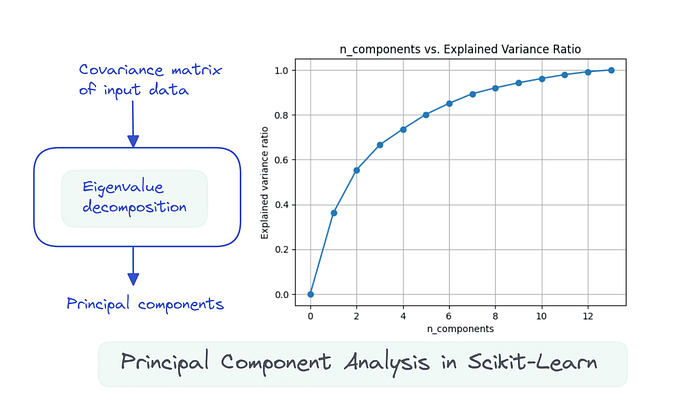
These percentages of variance can be visualized using Scree Plot.
Following figure plots variance ratios against each principal components

Selecting the Right Number of dimensions
The number of principal components is equal to the number of features in a dataset. The final goal is to reduce the dimensions in a dataset. Meaning n principal components need to be selected from a set of N components. Now how to choose the right number of n? Scree plot helps to select n.
Consider the below scree plot,

from the plot above we can understand that components PC1 , PC2 , PC3 and PC4 has much higher variance ratios , therefore carries more information. Also, the variance ratio decreasing scale became stable from PC5 onwards. Hence we can choose PC1, PC2, PC3, and PC4 as the final set of dimensions for the dataset, therefore n=4.

How to find PCAs in python?

sklearn.decomposition.PCA finds principal components from an N-dimensional dataset.

We will find principal components from KDD 2009 large dataset. Before performing PCA, we will execute below preprocessing steps,

1. Missing Value Filter: features with a missing value greater than 90% will be removed.
2. Missing Value Treatment: missing values in each numerical feature will be filled with the mean values.
3. Standardization: features will be standardized to bring all of them in a common range.
4. Finally will find Principal components and will select n high variance principal components.

Code Snippet

reduced_dataset has a shape of (50000, 5). (Note: Only the numerical features have been transformed into 5-dimensional space using PCA).